Analog Circuits

Lesson 2.1: Superposition with Dependent Sources

>A lot of textbooks say you can't do this. You can, though, as long as you don't calculate any values before summing all the individual solutions. You can't typically get a Thévenin or Norton equivalent directly with this technique. You'll have to solve the circuit first, then figure out what the Thévenin/Norton equivalents are.

This is Problem 5.76 from Basic Engineering Circuit Analysis, 11th edition, by Irwin and Nelms. (If you just want the worked solution on paper without reading through this, here you go.)

Here's an executive summary of what we're going to do.

Find the individual contribution of each source to the output. So turn off all other sources except the one you're interested in. ("Turning off" means shorting voltage sources and opening current sources.)
Sum up the individual contributions of each source to form the full output.

Warning: Do not try to calculate any numbers with the solutions for each individual source. You'll get the wrong answer. At least, you'll definitely get the wrong answer for the dependent source's equation alone. But wait, why is this? It's because you don't know how the dependent source will affect the circuit until you can solve for it. And you can't solve for it until you have all the necessary equations ready to go.

Let's assign symbols to all the circuit elements first, so we don't have to worry about which numbers are which.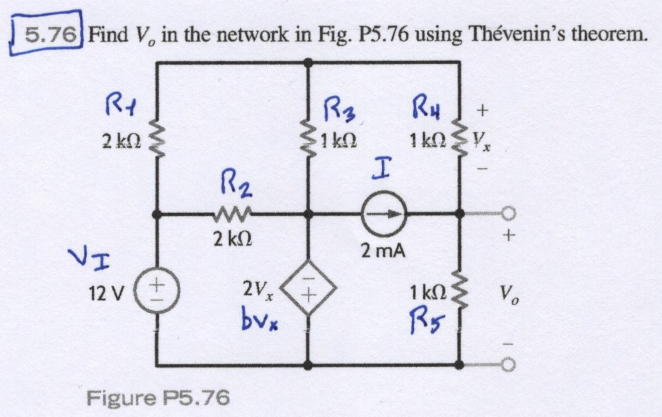 Circuit describing the problem.

(Assigning symbols to all elements.)

Next, we need to find the individual contribution of each source. I'll start with $ V_I $ alone. I'll refer to the positive side of the voltage $ V_x $ as $ V_{xp} $. This will be used later to calculate $ V_o $. We can ignore $ R_2 $ for now, since it doesn't really contribute to $ V_{xp} $. Writing the equations by inspection at the $ V_{xp} $ node.

$Assessing $ V_I $'s contribution.$

(Assessing $ V_I $'s contribution.)

\[ \frac{V_{xp}}{R_1 \parallel R_3 \parallel \left( R_4 + R_5 \right)} = \frac{V_I}{R_1} \] Solving for $ V_{xp} $. \[ V_{xp} = \frac{V_I}{R_1} \left[ {R_1 \parallel R_3 \parallel \left( R_4 + R_5 \right)} \right] \] The dependent source actually depends on the voltage across $ R_4 $, that is, $ V_x = V_{xp} - V_{xn} $. So we'll also need the solution for the negative side of $ V_x $, i.e., $ V_{xn} $. It's just a voltage divider of $ V_{xp} $ in this case. \[ V_{xn} = V_{xp} \frac{R_5}{R_4 + R_5} \]

On to the contribution of the dependent source $ b V_x $. It's actually pretty similar to the contribution of $ V_I $. Now the "supplied" or "current in" side is negative, though.

(Assessing $ b V_x $'s contribution.)

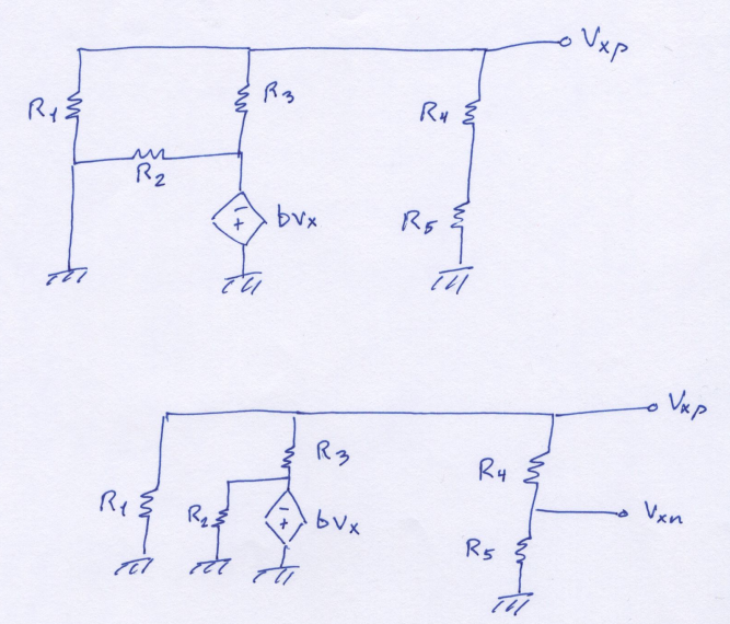
At node $ V_{xp} $, we can write \[ \frac{V_{xp}}{R_1 \parallel R_3 \parallel \left( R_4 + R_5 \right)} = -\frac{b V_x}{R_3}. \] Solve for $ V_{xp} $ once again: \[ V_{xp} = -\frac{b V_x}{R_3} \left[ {R_1 \parallel R_3 \parallel \left( R_4 + R_5 \right)} \right]. \] As before, $ V_{xn} $ is a voltage divider of $ V_{xp} $. The same one, in fact, written as \[ V_{xn} = V_{xp} \frac{R_5}{R_4 + R_5}. \]

Now we find the contribution of just the current source, $ I $. This one is a little more involved because the topology is different. After removing the sources, the circuit can be rearranged to simplify things.

(Assessing the contribution of $ I. $)

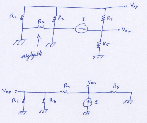
Using node $ V_{xn} $ is more powerful this time. \[ I = \frac{V_{xn}}{\left( R_1 \parallel R_3 \right) + R_4} + \frac{V_{xn}}{R_5} \] \[ I = \frac{V_{xn}}{\left[ \left( R_1 \parallel R_3 \right) + R_4 \right] \parallel R_5} \] Solve for $ V_{xn} $. \[ V_{xn} = I \left[ \left( R_1 \parallel R_3 \right) + R_4 \right] \parallel R_5 \] $ V_{xp} $ is a divided voltage of $ V_{xn} $. \[ V_{xp} = V_{xn} \frac{ \left( R_1 \parallel R_3 \right) }{ \left( R_1 \parallel R_3 \right) + R_4 } \]

Using the fact that $ V_x = V_{xp} - V_{xn} $, the solutions for $ V_{xp} $ fall out.

$ V_1 $ alone $ \rightarrow V_{xp,1}. $ \[ V_{xp} = \frac{V_I}{R_1} \left[ {R_1 \parallel R_3 \parallel \left( R_4 + R_5 \right)} \right] \left( 1 - \frac{ R_5 }{ R_4 + R_5 } \right) \] $ b V_x $ alone $ \rightarrow V_{xp,2}. $ \[ V_{xp,2} = -\frac{b V_x}{R_3} \left[ {R_1 \parallel R_3 \parallel \left( R_4 + R_5 \right)} \right] \left( 1 - \frac{ R_5 }{ R_4 + R_5 } \right) \] $ I $ alone $ \rightarrow V_{xp,3}. $ \[ V_{xp,3} = I \left( \left[ \left( R_1 \parallel R_3 \right) + R_4 \right] \parallel R_5 \right) \left( \frac{ \left( R_1 \parallel R_3 \right) }{ \left( R_1 \parallel R_3 \right) + R_4 } - 1 \right) \]

Apply superposition. Solve for $ V_{xp} $. \[V_{xp} = V_{xp,1} + V_{xp,2} + V_{xp,3} \] $ V_{xp,2} $ is the only term besides $ V_{xp} $ on the left side that includes a $ V_{xp} $ variable. \[V_{xp} - V_{xp,2} = V_{xp,1} + V_{xp,3} \] Expanding the left-hand side. Factoring $ V_{xp} $ out. \[V_{xp} \left( 1 + \frac{b}{R_3} \left[ {R_1 \parallel R_3 \parallel \left( R_4 + R_5 \right)} \right] \left( 1 - \frac{ R_5 }{ R_4 + R_5 } \right) \right) = V_{xp,1} + V_{xp,3} \]

This equation will get really messy if we write out the whole thing. I'll define two new resistance terms to clean it up. \[ R_a = R_1 \parallel R_3 \parallel \left( R_4 + R_5 \right) \] \[ R_b = \left[ \left( R_1 \parallel R_3 \right) + R_4 \right] \parallel R_5 \] Here's the final solution for $ V_{xp} $. \[ V_{xp} = \frac{\frac{ V_I }{ R_1 } R_a \left( 1 - \frac{ R_5 }{ R_4 + R_5 } \right) + I R_b \left[ \frac{ \left( R_1 \parallel R_3 \right) }{ \left( R_1 \parallel R_3 \right) + R_4 } - 1 \right]}{ 1 + \frac{b}{R_3} \left[ {R_1 \parallel R_3 \parallel \left( R_4 + R_5 \right)} \right] \left( 1 - \frac{ R_5 }{ R_4 + R_5 } \right)} \]

We have to return to the original circuit to find the solution for $ V_o $.

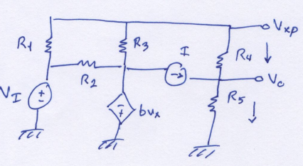
$Finding Vo using the solution we just got for Vxp. \)$

Finding $ V_o $ using the solution we just got for $ V_{xp} $.

Writing a KCL equation at node $ V_o $ yields \[ \frac{ V_{xp} - V_o }{ R_4 } + I = \frac{ V_o }{ R_5 } \] and \[ V_o = \left(\frac{ V_{xp} }{ R_4 } + I \right) \left(R_4 \parallel R_5 \right) \]

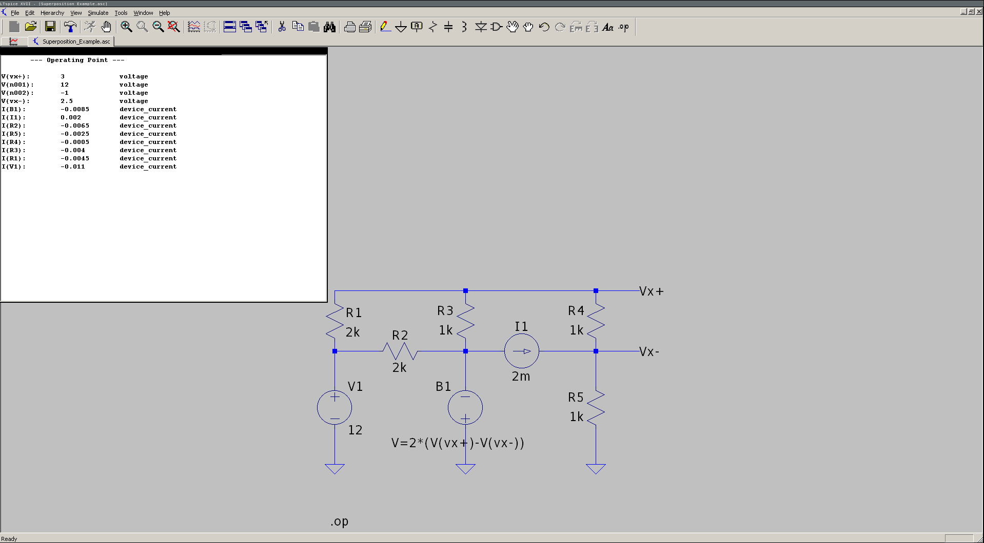
Let's start plugging in numerical values. \[ R_a = 2 \text{k} \parallel 1 \text{k} \parallel \left( 1 \text{k} + 1 \text{k} \right) = 500.00 ~Ω \] \[ R_b = \left[ \left( 2 \text{k} \parallel 1 \text{k} \right) + 1 \text{k} \right] \parallel 1 \text{k} = 625.00 ~Ω \] \[ V_{xp} = \frac{\frac{ 12 }{ 2 \text{k} } (500) \left( 1 - \frac{ 1 \text{k} }{ 1 \text{k} + 1 \text{k} } \right) + (2 ~\text{mA}) (625) \left[ \frac{ \left( 2 \text{k} \parallel 1 \text{k} \right) }{ \left( 2 \text{k} \parallel 1 \text{k} \right) + 1 \text{k} } - 1 \right]}{ 1 + \frac{2}{1 \text{k}} (500) \left( 1 - \frac{ 1 \text{k} }{ 1 \text{k} + 1 \text{k} } \right)} = 3.00753 ~\text{V} = 3.00 ~\text{V} \] Plug that into the expression for $ V_o $. \[ V_o = \left( \frac{ 3.00753 ~\text{V} }{ 1 \text{k} } + 2 ~\text{mA} \right) \left( \frac{ 1 \text{k} }{ 1 \text{k} + 1 \text{k} } \right) = 2.5038 ~\text{V} = 2.50 ~\text{V} \] These values are dangerously close to what you'd get simulating this circuit with LTSpice.

(Checking the numbers with LTSpice.)

As you can see, the solution we got from this method was huge. That's okay, though; the final expression is modular. So if you messed up some portion of the solution, you only need to fix that portion, and no other.

You can read more about this technique in William Leach's unpublished paper on it.. It has tons of examples, so you can use those to check your understanding. You can also take a look at the StackExchange post where I originally found that paper.

If you found this content helpful, it would mean a lot to me if you would support me on Patreon. Help keep this content ad-free, get access to my Discord server, exclusive content, and receive my personal thanks for as little as $2. :)

Become a Patron!