
Signals and Systems

Lesson 1: Playing with Sinewaves
The Humble Sinewave
Ah, the humble sinewave. You have likely already met this beast in other coursework, or in a trigonometry course in primary school. In this class, we are going to get to know it much more intimately. The goal of this lesson is for you to learn to dance with the sinewave - scale, shift, and squeeze it, and understand the basic terminology we use to describe it.
First, the most basic version, the one you are probably familiar with, \(sin(x) \), Here, \(x\) is what is called the "total phase" of the sinewave, or "phase" for short. We can plot this equation versus x, and we get your garden-variety sinewave:
 The most interesting parts of the sinewave are that it goes from -1 to +1, it is zero at every integer value of \(\pi\), and it is periodic, meaning it repeats itself. In this case, the period of the sinewave is equal to \(2\pi\), since this sinewave repeats itself after we increase the value of \(x\) by \(2\pi\). Notice that in this case, the period is in radians, and doesn't have units of time.
Time versus pure radians
For most of this course, we will be dealing with functions not of \(x\), but of time (although it will sometimes be convenient to switch back and forth). You might think we write those sinewaves like \(sin(t)\), but then we would have to take the sin() of something with units of seconds, and I'm not sure how to do that. For this reason, sinewaves that are functions of time we write as \(sin(\omega t)\), where \(\omega\) is called the "angular frequency", and has units of radians per second. That way, when we multiply \(\omega *t\), we get something in radians, and that I know how to plug into a sin() function! This is a common confusion that trips people up.
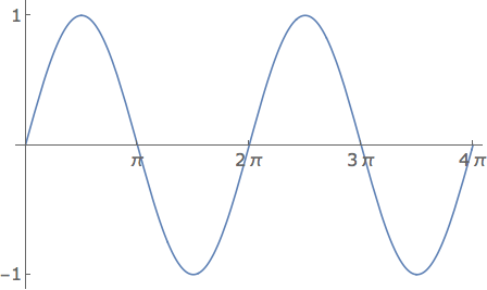
For example, if we had an angular frequency of \(2\pi\) per second, we could plot that sinewave (to the right).
 Now, instead of radians on the x-axis, we have time, in units of seconds. When the time is equal to 1 second, the total phase of the sinewave \(\omega*t\) is equal to \(2\pi\) / second * \(1\) second \(= 2 \pi\), and the sinewave will have value 0. When time is equal to 0.25 seconds, the phase will be \(\pi/2\), and the sinewave will have a value of 1.
Angular Frequency, Period, and Frequency
You might be more comfortable and familiar with the period of a sinewave, rather than the angular frequency. We can use either, and since we know that a sinewave repeats itself every time the phase is \(2\pi\), that means that when we plug in one period for \(t\) (let's call it \(T\)), we should get \(2\pi\).
\(\omega T = 2\pi\)
or
\(T = 2\pi / \omega \)
This relates the period of the sinewave and the angular frequency. You might be wondering why we are going through all the trouble of using angular frequency instead of just using the period directly - the period seems like something more physically meaningful - the time after which the signal repeats itself. The main reason has to do with derivatives and integrals. We will be taking lots of both of these, and it's very convenient writing \(sin(\omega t)\), because it's derivative is \(\omega * cos(\omega t)\), rather than \(sin(2\pi t/T)\), whose derivative is \(2\pi /T * sin(2 \pi t / T)\). You can see how after one or two derivatives things can get very messy very quickly.
We also sometimes care about the regular frequency (we will use the symbol \(f\), for frequency). This is the number of times per second the signal repeats itself, and because it is used so often, it gets its own unit, the Hertz. A sinewave that repeats itself twice in one second has a frequency of 2\(Hz\). In order to repeat itself twice in one second, the period must be 0.5s. In general, the period, in seconds, must be 1 / (# periods per second), or \(1/f\).
You might ask - what happens when we increase the frequency? What does the sinewave look like? For example, what happens when we double the frequency?

As you might have guessed, if we plot the function over the same amount of time, we have twice as many periods. Or, if we felt so inclined, we could say the sinewave is changing "twice as fast" (this is actually exactly true if you compute the derivative, it will be twice as large - check!). Frequency (angular or regular) is thus a measure of the speed of the signal, how rapidly it changes in time. Higher frequency → faster signal. Lower frequency → slower signal. This theme will recur over and over again. If we wanted to also plot a sinewave at half the frequency, we see that there are fewer periods (only one in two seconds), and it is changing more slowly with time:

Now to give you some practice mastering the material, I have posted a few practice questions below.
If \(\omega = 6\pi\) rad/s, what is the period T?
If \(T = 0.2s\), what is \(f\)?
If a sinewave period halves, what happens to the angular frequency?
If a sinewave frequency doubles, what happnes to the angular frequency?
If you found this content helpful, it would mean a lot to me if you would support me on Patreon. Help keep this content ad-free, get access to my Discord server, exclusive content, and receive my personal thanks for as little as $2. :)
Become a Patron!