
Computational Electromagnetics with MEEP: 1D MEEP

Lesson 12: Resonators
It's Just two mirrors...
In the last lesson we went over how to create Bragg reflectors in MEEP, which act like really really good mirrors over a narrow range of frequencies. This allows us to create another very cool object - the resonator. Resonators are ubiquitous in electromagnetics and optics. Waveguide? That's a resonator. Want to make a filter? You can do that with a resonator. Need to make a laser? You'll need a resonator for that. In its simplest form, a resonator is just two mirrors (reflecting surfaces) separated by some distance. You can think of a thin film as a resonator, just a pretty bad one, because the mirrors have such low reflectivities.

Often with resonators what we're after for is the transmittance or reflectance spectrum - we want to known \(R\) as a function of frequency. Fortunately, we know how to do this now and have done it several times. All we need to do is send in our finite-duration, bandwidth-limited (gaussian) pulse, and then have MEEP do all the heavy Fourier Transforming for us. Let's modify the code from the previous lesson, adding in a resonant cavity (of width 0.5 and index 1), and another 8-layer mirror. So our layer indexes and thicknesses should look like this:
layerIndexes = np.array([1.0, n1, n2, n1, n2, n1, n2, n1, n2, n1, 1, n1, n2, n1, n2, n1, n2, n1, n2])
layerThicknesses = np.array([5, t1, t2, t1, t2, t1, t2, t1, t2, t1, 0.5, t1, t2, t1, t2, t1, t2, t1, t2])
Neat! Now all we have to do is run the simulation. Let's get started. First, I'm going to narrow the frequency to be from 1.5 to 2.5 (MEEP units), since this will cover a single 'period' of our periodic reflectance spectra (see the previous lesson), and this lets us reduce the resolution from 120 to 40. Let's run the simulation.
Tick tock, tick tock
What on earth is taking so long? My simulation is at took over 3600 MEEP units to run (after I disabled the updateField line so that this wouldn't take a full day). Let's take a look inside the simulation to end at a particular time and see what's going on. I tried a few different end times, but 80 seems to be enough to see what is going on. Take a look (or try it yourself, either by modifying the code or downloading it here):
What is a 'mode', anyway?
That's some fascinating behavior right there. It looks like the wave cames in, most of it reflects back as expected, but some of it gets inside the resonator, and seems to get stuck there (hence the name 'resonator'). It slowly bleeds off more and more amplitude until it looks purely like a standing wave inside the resonator, slowly leaking outward. This standing wave pattern is called a mode and is plenty interesting in its own right.
Let's just take a moment to appreciate how difficult this would have been to do by hand - theoretically possible, but only if you're okay with your equations being pages and pages long. We are finally at the point where FDTD is paying serious dividends, and we haven't even left one dimension yet.
So, what about the reflection spectra? Well, if you plot it with 200 frequency points, it looks something like this:

Does this make sense?. Well, it looks very similar to what we saw in the previous lesson, with the almost-1 (I'm getting about \(0.99995\)) reflectance near the maxima at \(f=1\). This makes sense, because we're basically cascading two mirrors after each other, so we expect an absurdly high reflectance. And what about that small dip in the middle? Well, that is at exactly the frequency we expect of the mode that gets stuck inside the resonator. But why is the dip so small? If you zoom in on it, you will see it is just a single point, so that's probably not accurate. Let's zoom in on that part of the graph by setting our frequency width to 0.01 and re-running the simulation.

Now, does this make sense? Well, the minimum frequency is a little off, but I suspect that's due to our low resolution of 8 points per wavelength and could be fixed with some convergence testing. The dip goes pretty darn close to 0, and (I was trying to figure out why this wasn't happening the first time I tried this) this has to do with the symmetry of the mirrors - since they each have the same reflectance, this is the expected behavior. If they were asymmetric, this would not be the case.
But these simulations are starting to take a really long time. And this is just 1 dimension - what happens when we start to run 2D and 3D simulations? How are we going to deal with such structures?
Cheating cheaters
The answer is that we cheat. If we are interested in the full reflectance spectra, with all its subtleties, sure, we would just have to suck it up run a long and painful simulation. But if we are only interested in what is happening near the resonant frequency, as is often the case, then it turns out all of our analysis boils down to three things - the resonant frequency \(f\), the quality factor \(Q\), and the magnitude of the dip.
 For symmetric mirrors, this last one will be 1 (the reflectance goes from near \(1\) to \(0\)), and we can usually find this quantity by hand. The only things we need to find is the resonant frequency and the quality factor. Once we know the resonant frequency, we know where we should see the dip. Once we know the quality factor, we know how wide the dip should be (\(Q\) is defined to be the resonant frequency \(f\)divided by the full-width-half-max \(\Delta f\) of the dip). And because Maxwell's equations are linear and modes decay exponentially in time, we know the shape of the curve - it's a Lorentzian.
What is the quality factor (roughly) of the mode we just found above?
MEEP Saves the Day
Because of the fact that we already know so much about the behavior near resonance of the curve, we don't actually need to run a very long simulation at all. MEEP actually provides some extremely efficient algorithms to give us the resonant frequency and the quality factor of these types of structures. Instead of running our simulation until the fields decay to some predefined threshold (we have been using \(10^{-9}\)), we wait until after the sources have died out, and then tell MEEP to perform a 'harmonic inversion'. The code to actually do that for our simulation looks like this:
simulation.run(
        mp.after_sources(mp.Harminv(mp.Ex, mp.Vector3(0, 0, layerCenters[10]), frequency, frequencyWidth)),
        until_after_sources=400)
This waits until 400 MEEP units after the sources have been turned off (sources can really mess with stuff if they don't get turned off before the harmonic inversion). Let's run this code again, and use frequencies from 0.5 to 1.5 once more, and let's run the code without the reflectance plot and animations, just to see what Harminv gives us. Let's also drop the resolution down to 40 to see if Harminv is affected by the same convergence issues as our normal simulation. You can find the code to do this here.
Wow! That was blazingly fast. It took my computer about 2 seconds to run, and this is the output I get from harminv:
harminv0:, frequency, imag. freq., Q, |amp|, amplitude, error
harminv0:, 0.6968858245597717, -0.005671653242234428, 61.435863124560804, 0.009716561746302916, -0.006731411467840067-0.007007115798982374i, 0.002513852795880678+0.0i
harminv0:, 0.9981896877871808, -0.0003344723861172638, 1492.1854975454119, 0.03983516871781626, 0.0005814049751895879+0.03983092561103385i, 1.1079276290101826e-07+0.0i
We see two apparent resonant frequencies - since our bandwidth was so large, it looks like MEEP picked up one of extra dips on the side of our reflection spectra. The second line, though, contains what we expect. A resonant frequency at 0.998 (almost excatly what we see in the zoomed-in non-converged figure above), and a quality factor of 1492, a little less than expected. Let's do some convergence testing and see how this affects things, by doubling the resolution.
If I double the resolution once (to 80), I get the following output from Harminv:
harminv0:, frequency, imag. freq., Q, |amp|, amplitude, error
harminv0:, 0.9995505429370294, -0.0003168792947367963, 1577.1786916012736, 0.03892037556354569, 0.0004933889669062501+0.038917248121299375i, 1.517651217154188e-08+0.0i
run 0 finished at t = 410.0 (65600 timesteps)
Looks like it realized the second mode it gave us was a mistake - not actually a mode. That's really good to know - if the simulation isn't converged, we can pick up modes that aren't even there! The quality factor is also closer to what we expect, at 1577. Doubling the resolution again gets us to 1602, and again to 1609. So I would be pretty confident with a \(Q\) of around 1600, very close to what we got from visual estimation.
All the wasted energy!
You might now be wondering - if all we're interested in is the single mode near a frequency of 1, is there a way to 'turn on' that made all by itself? Right now, we're sending in a plane wave from the left, and most of it bounces back and out of the simulation domain. Only a very small amount actually gets inside the resonator and lets Harminv do its thing. That seems like an awful waste if we aren't trying to simulate reflection spectra directly. And what if the mirrors were even more reflective? We would get even less energy into the cavity, and eventually we might not get enough to do our simulation! In any case, this seems like an awfully wasteful way of doing things.
Source inside the cavity
Instead we can do something clever - we can put the source inside the cavity. This prevents all the energy from being wasted through reflection, and is an easy way of getting a large amount of energy inside the resonator. Now, this would be quite impossible to do in reality, but since this is a simulation we can put our sources wherever we please. If we change our source location to be the center of the 11th layer, we can do exactly this:
sourceLocation = mp.Vector3(0, 0, layerCenters[10])
Now let's plot it (full code here) to make sure everything looks as we expect:
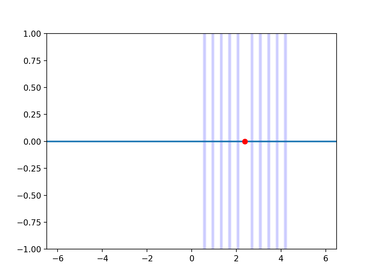
Perfect! The source (the red dot) is right in the center of our resonator, just as we wanted. If we run this simulation, we see that we converge to a quality factor of ~1600 in a similar fashion to the previous simulation. So for this case, exciting the mode directly by placing the source inside the cavity didn't seem to give us any benefit, but for structures of higher quality factors the improvement can be significant. What about the mode itself, or the fields oscillating in time? Can we still see these if we use Harminv and terminate the simulation early? Well, yes. All we need to do is plot the field versus time near the end of the simulation. The easiest way to do this is probably just to run another simulation. Let's run it for two periods of oscillation and sample it at 80 times per period, outputting the field as we have done before using updateField().
simulation.run(mp.at_every(1/frequency/80, updateField), until=2/frequency)
You might notice here (depending on the frequency width you use to excite the mode) that the fields are actually too large to visualize using the limits we have bee nusing from -1 to 1. We can change the limits of our plots by finding the maximum value of our data:
yLimit = fieldData.max() + 1
ax = plt.axes(xlim=(min(z),max(z)),ylim=(-yLimit,yLimit))
We will also have to change the limits for showing our refractive index, changing the line with fill_between to include the limit in the y direction of the plot:
ax.fill_between([z[i], z[i+1]], [-yLimit, -yLimit], [yLimit, yLimit],
Great! Now if we run the simulation and check out the animation, what do we see?
Woah! This is what the electric field of our mode looks like - very high amplitude in the center, and decaying off to the sides. We can also see it leaking away into the surrounding space, and this is expected, because it has a finite lifetime. What if we zoom in on just the center region of the resonator, including only the \(n=1\) layer where the field is strongest?
Notice that it's almost a perfect standing sinewave. The field at the edges is very close to zero for the entire period of oscillation. This is exactly the mode profile that we see in resonators with perfectly conducting boundaries - where the electric field must go to zero at the boundaries - it's almost as if we can 'lump' our dielectric mirrors into a single highly reflecting element, where the field at the edges decays to almost zero. This is actually a very productive way of thinking about resonators.
What's next?
We have now gone over most of what MEEP (and any FDTD simulator, really) can do in one dimension. While there is certainly more fun to be had (anti-reflection coatings, resonant frequencies and quality factors at an angle, and so on), we now know enough to set up simulations and experiment ourselves. Next we are going to start MEEP in two dimensions, where even more interesting things start happening (and we can generate some really pretty graphics!)
Full Code
You can find the full code for finding the quality factors and plotting the mode here. The code for plotting reflectance spectra and positioning the source prior to the resonator is commented out.
import meep as mp
import numpy as np
import matplotlib.pyplot as plt
from matplotlib import animation

resolution = 40
frequency = 1.0
frequencyWidth = 0.01
numberFrequencies = 200
pmlThickness = 2.0
animationTimestepDuration = 0.1
powerDecayTarget = 1e-9
t1 = 0.125
t2 = 0.25
n1 = 2.0
n2 = 1.0
ns = 1.3
ts = 0.2
endTime = 80;

layerIndexes = np.array([1.0, n1, n2, n1, n2, n1, n2, n1, n2, n1, 1, n1, n2, n1, n2, n1, n2, n1, n2, n1, n2])
layerThicknesses = np.array([5, t1, t2, t1, t2, t1, t2, t1, t2, t1, 0.5, t1, t2, t1, t2, t1, t2, t1, t2, t1, t2])
layerThicknesses[0] += pmlThickness
layerThicknesses[-1] += pmlThickness
length = np.sum(layerThicknesses)
layerCenters = np.cumsum(layerThicknesses) - layerThicknesses/2
layerCenters = layerCenters - length/2

#sourceLocation = mp.Vector3(0, 0, layerCenters[0] - layerThicknesses[0]/4)
sourceLocation = mp.Vector3(0, 0, layerCenters[10])
transmissionMonitorLocation = mp.Vector3(0, 0, layerCenters[-1]-pmlThickness/2)
reflectionMonitorLocation = mp.Vector3(0, 0, layerCenters[0] + layerThicknesses[0]/4)

cellSize = mp.Vector3(0, 0, length)

sources = [mp.Source(
    mp.GaussianSource(frequency=frequency,fwidth=frequencyWidth),
    component=mp.Ex,
    center=sourceLocation)
    ]

geometry = [mp.Block(mp.Vector3(mp.inf, mp.inf, layerThicknesses[i]),
    center=mp.Vector3(0, 0, layerCenters[i]), material=mp.Medium(index=layerIndexes[i]))
    for i in range(layerThicknesses.size)]

pmlLayers = [mp.PML(thickness=pmlThickness)]

simulation = mp.Simulation(
    cell_size=cellSize,
    sources=sources,
    resolution=resolution,
    dimensions=1,
    boundary_layers=pmlLayers)

incidentRegion = mp.FluxRegion(center=reflectionMonitorLocation)
incidentFluxMonitor = simulation.add_flux(frequency, frequencyWidth, numberFrequencies, incidentRegion)

simulation.run(until_after_sources=mp.stop_when_fields_decayed(20, mp.Ex,
    transmissionMonitorLocation, powerDecayTarget))

fieldEx = np.real(simulation.get_array(center=mp.Vector3(0, 0, 0), size=cellSize, component=mp.Ex))
fieldData = np.zeros(len(fieldEx))

incidentFluxToSubtract = simulation.get_flux_data(incidentFluxMonitor)

simulation = mp.Simulation(
    cell_size=cellSize,
    sources=sources,
    resolution=resolution,
    boundary_layers=pmlLayers,
    dimensions=1,
    geometry=geometry)

transmissionRegion = mp.FluxRegion(center=transmissionMonitorLocation)
transmissionFluxMonitor = simulation.add_flux(frequency, frequencyWidth, numberFrequencies, transmissionRegion)
reflectionRegion = incidentRegion
reflectionFluxMonitor = simulation.add_flux(frequency, frequencyWidth, numberFrequencies, reflectionRegion)
simulation.load_minus_flux_data(reflectionFluxMonitor, incidentFluxToSubtract)

def updateField(sim):
    global fieldData
    fieldEx = np.real(sim.get_array(center=mp.Vector3(0, 0, 0), size=cellSize, component=mp.Ex))
    fieldData = np.vstack((fieldData, fieldEx))

simulation.run(
        mp.after_sources(mp.Harminv(mp.Ex, mp.Vector3(0, 0, layerCenters[10]), frequency, frequencyWidth)),
        until_after_sources=400)

simulation.run(mp.at_every(1/frequency/80, updateField), until=2/frequency)

incidentFlux = np.array(mp.get_fluxes(incidentFluxMonitor))
transmittedFlux = np.array(mp.get_fluxes(transmissionFluxMonitor))
reflectedFlux = np.array(mp.get_fluxes(reflectionFluxMonitor))
R = -reflectedFlux / incidentFlux
T = transmittedFlux / incidentFlux
#print(T)
#print(R)
#print(R + T)

#frequencies = np.array(mp.get_flux_freqs(reflectionFluxMonitor))
#reflectionSpectraFigure = plt.figure()
#reflectionSpectraAxes = plt.axes(xlim=(frequency-frequencyWidth/2, frequency+frequencyWidth/2),ylim=(0, 1))
#reflectionLine, = reflectionSpectraAxes.plot(frequencies, R, lw=2)
#reflectionSpectraAxes.set_xlabel('frequency (a / \u03BB0)')
#reflectionSpectraAxes.set_ylabel('R')
#plt.show()

(x, y, z, w) = simulation.get_array_metadata()
indexArray = np.sqrt(simulation.get_epsilon())
print(fieldData[-1])

fig = plt.figure()
yLimit = fieldData.max() + 1
ax = plt.axes(xlim=(min(z),max(z)),ylim=(-yLimit,yLimit))
line, = ax.plot([], [], lw=2)

colorArray = indexArray - 1 # make sure free space shows up as white
if(colorArray.max() > 0):
    colorArray = colorArray / colorArray.max() # normalize the color array so that the max index shows up dark blue
for i in range(len(indexArray) - 1):
    ax.fill_between([z[i], z[i+1]], [-yLimit, -yLimit], [yLimit, yLimit],
            color=(1-colorArray[i],1-colorArray[i],1), linewidth=0.0, alpha=0.2)
ax.plot(sourceLocation.z, 0, 'ro')
#ax.axvline(transmissionMonitorLocation.z, ymin=-1, color='black')
#ax.axvline(reflectionMonitorLocation.z, ymin=-1, color='black')

def init():
    line.set_data([],[])
    return line,

def animate(i):
    line.set_data(z, fieldData[i])
    return line,

numberAnimationTimesteps = fieldData.shape[0]
fieldAnimation = animation.FuncAnimation(fig, animate, init_func=init,
        frames=numberAnimationTimesteps, interval=20, blit=True)

#fieldAnimation.save('basic_animation.mp4', fps=30, extra_args=['-vcodec', 'libx264'])
plt.show()
If you found this content helpful, it would mean a lot to me if you would support me on Patreon. Help keep this content ad-free, get access to my Discord server, exclusive content, and receive my personal thanks for as little as $2. :)
Become a Patron!