
Computational Electromagnetics with MEEP: 1D MEEP

Lesson 11: Distributed Bragg Reflectors
Distributed Bragg Reflector
The dielectric mirror (also known as the Bragg Mirror, or Bragg Reflector, or Distributed Bragg Reflector), is an awesome idea. Loosely speaking, it says if one film can give us constructive interference, maybe more films give us better constructive interference. OK, let's pick up where we left off in the previous lesson. We did an experiment with a plane wave incident on a single thin film, and we observed maxima and minima where we expected. Let's just add more films! This will look something like the figure below:

Where I have shown three pairs of material alternating between high index (shown in orange), and low index (shown in blue). To make things easy on ourselves, let's say the blue regions have an index of 1 and the orange regions have an index of 2. Let's keep everything else as in the previous simulation, with a center frequency of 4 and a bandwidth of 7. This will let us observe multiple interference maxima and minima.
Where is everything?
When we just had a single interface to deal with, it was simple enough to make sure everything was working as expected - we know the interface is there just by seeing reflection from it. But now that we have multiple layers, it becomes much more challenging to see what is actually going on with the fields, much less whether we have set up our geometry correctly. Unfortunately (as of this writing), MEEP doesn't provide built-in functionality to visualize 1D simulations, so we're going to have to implement our own. We will be using matplotlib for this. If you're confused about all the plt.figure() and plt.axes() commands flying around and want to learn more, there's an excellent tutorial on Real python that goes over matplotlib, which I won't discuss in-depth here.
To make sure we are setting everything up correctly, we need to ask MEEP where everything is. In other words, we need to know what MEEP thinks the refractive index is everywhere throughout our simulation domain. Fortunately, MEEP's does have built-in methods for getting this information using get_epsilano(). This will give us an array that contains the permittivity at all points in the simulation. To map those points onto our spatial dimension, we can use the get_array_metadata() function, which grabs arrays that contain all our coordinates. Here are the actual lines of code (which need to be placed after we have set up / run our second simulation). We are working off the code fromm the code we developed at normal incidence, because that's what we will be working with for the time being (just to simplify things), with some slight quality-of-life modifications (and don't worry, as usual the full code will be posted below).
(x, y, z, w) = simulation.get_array_metadata()
indexArray = np.sqrt(simulation.get_epsilon())
Now, how might we visualize this? Ideally, we'd like to overlay it directly on top of our field plot, so we can watch the field as it propagates through the various layers. First, we need to map all the refractive indices into colors. Since I like the color blue, I'm going to plot everything in blue, and say that anywhere white should be the color of free space. The color code for pure white is (1, 1, 1) in RGB and the color code for pure blue is (0, 0, 1). So the highest index on the plot I want to be pure blue, and free space should be white. The following code creates an array of how blue we want everything to be, from 0 to 1.
colorArray = indexArray - 1 # make sure free space shows up as white
if(colorArray.max() > 0):
    colorArray = colorArray / colorArray.max() # normalize the color array so that the max index shows up dark blue
Finally, we are going to actually color the plot, using matplotlib's fill_between() method, which just fills everything in a polygon whose boundaries you define. 'alpha' is just matplotlib's way of creating transparency, and linewidth=0 makes sure we see a continuous smooth color instead of a bunch of blocks.
for i in range(len(indexArray) - 1):
    ax.fill_between([z[i], z[i+1]], [-1, -1], [1, 1],
            color=(1-colorArray[i],1-colorArray[i],1), linewidth=0.0, alpha=0.2)
Finally, if we want, we can add the location of our source (with a red dot) and our transmission monitors (with black vertical lines):
ax.plot(sourceLocation.z, 0, 'ro')
ax.axvline(transmissionMonitorLocation.z, ymin=-1, color='black')
ax.axvline(reflectionMonitorLocation.z, ymin=-1, color='black')
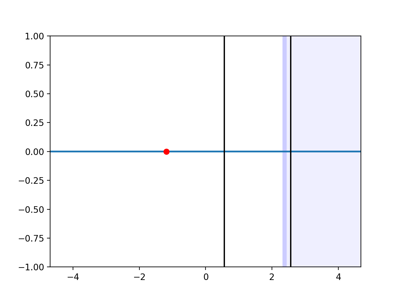
Let's just quickly run the code to see that our visualization is working as we expected, just for a simple interface. You can find that partial code here.
Beautiful! We see that the source is located exactly where we expect it, followed by the reflected power monitor, the interface, and the transmission monitor. We also see that the media extend the full range of the simulation, so there is no nonuniformity in our PMLs (and if we so desired we could add these to the plot, too!). You might notice something interesting at the boundary - it looks like there's some blurring going in. That's not an artifact of the plotting, that's real. MEEP uses subpixel smoothing to smooth out sharp interfaces, which help avoid 'staircaising' in 2D and 3D simulations (approximating a sphere as a bunch of cubes).
Defining the Mirror
Now that we have a way of seeing our geometry, we can move on to actually creating it. In this simulation we are going to start out with 3 layers as in the previous simulation (free space, our thin film, and our 'substrate' - just another name for the underlayer). While we could write all the thicknesses and locations of these explicitly like we have been doing, that's going to get very painful when we start adding more layers. Instead, we can define all the indexes of refraction, the thicknesses, and the centers at the very beginning of the code. Let's use the same thickness for the \(n=2\) film we were using in our previous simulation - a thickness of 0.125 MEEP units. For a film with half the refractive index \(n=1\), we will need a film twice as thick to get the same type of interference, so let's use a thickness of 0.25 for this film thickness.
n1 = 2.0
t1 = 0.125
n2 = 1.0
t2 = 0.25
layerIndexes = np.array([1, n1, n2])
layerThicknesses = np.array([5, t1, t2])
Now, remember that the PMLs need to be included in the layer closest to the edge, so we will expand the first and the last layers to accomodate the PMLs. Once we make this correction we can also compute the total length:
layerThicknesses[0] += pmlThickness
layerThicknesses[-1] += pmlThickness
length = np.sum(layerThicknesses)
Finally, we can compute the center of each layer. For the center of the first layer, we can choose whatever we like, but to make things simple let's say the simulation domain should start at a z-value of 0. That means the first layer should be centered at half its thickness. The second layer should be centered at the thickness of the first layer plus half its own thickness, and so on. Each layer should thus be located at the cumulative sum of all the previous layers, minus half its own thickness. Fortunately, this is just a one-liner in python:
layerCenters = np.cumsum(layerThicknesses) - layerThicknesses/2
Also, MEEP by default wants to put the center of the simulation at (0, 0, 0). So, for a given length in our simulations, MEEP expects the geometry to be between -length/2 and length/2. We can make sure this is true if we shift the center of our layers to (0,0,0) (or just by half the length, since we started them at \(z=0)).
layerCenters -= length/2
We are also going to have to change the location of our source and transmission and reflection monitors to make sure that they are in the appropriate locations. We just need to make sure that our reflection monitor is to the left of the interface (and not directly on top of the source), the transmission monitor is to the right of the interface, and none are inside the PMLs.
sourceLocation = mp.Vector3(0, 0, layerCenters[0])
reflectionMonitorLocation = mp.Vector3(0, 0, layerCenters[0] + layerThicknesses[0]/4)
transmissionMonitorLocation = mp.Vector3(0, 0, layerCenters[1])
Finally, now that we have defined the locations for everything, the only difference from our previous code is defining the geometry - we just need to loop over all the layers and add a layer at the desired location, with the desired thickness and the desired index. For this we can use a python list comprehension.
geometry = [mp.Block(mp.Vector3(mp.inf, mp.inf, layerThicknesses[i]),
    center=mp.Vector3(0, 0, layerCenters[i]), material=mp.Medium(index=layerIndexes[i]))
    for i in range(layerThicknesses.size)]
Whew! OK, now that we've made these quality-of-life enhancements to our code, we're ready to actually run it and see what happens. You can find this partial code for just one layer here. We should see the same exact thing we saw in the previous simulation, with minima at frequencies of 2, 4, an 6 and maximas at 1, 3, 5, and 7. Let's plot the reflection spectra and our fields and make sure everything looks like we expect:
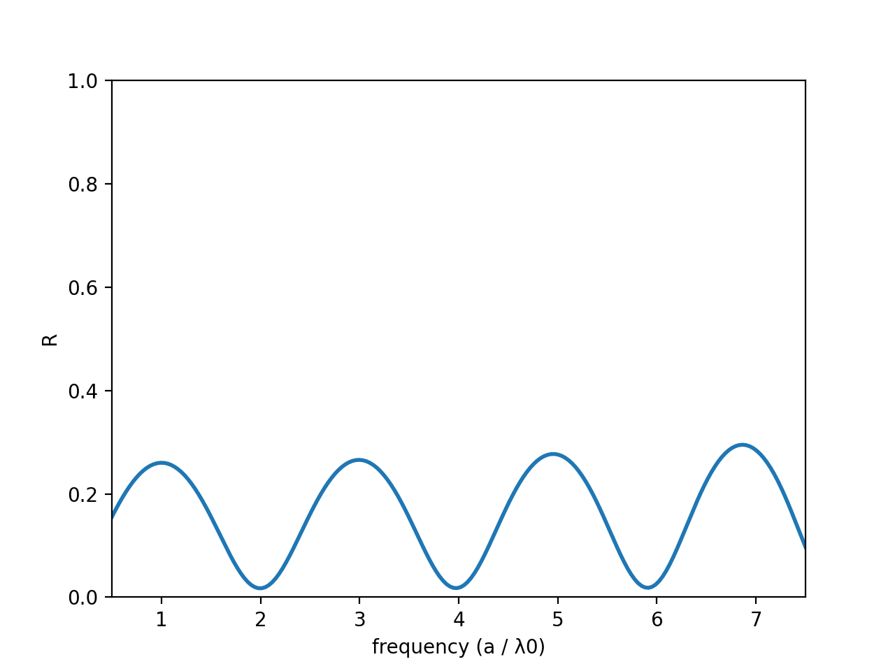
Do these results make sense? Well, yes, the monitors and the sources appear to be exactly where we want them, and the spectra looks exactly the same as in the last simulation. Our maxima aren't exactly where we expect them, and some are taller than others, but we now know that's just a convergence artifact. Now let's add a couple of layers. The beauty of the code we have written is all we need to do is change our layerIndexes and layerThicknesses:
layerIndexes = np.array([1.0, n1, n2, n1, ns])
layerThicknesses = np.array([5, t1, t2, t1, ts])
Now we can run the simulation again and see what happens. If we plot the reflection spectra, we see the maxima are a lot higher than they were before:
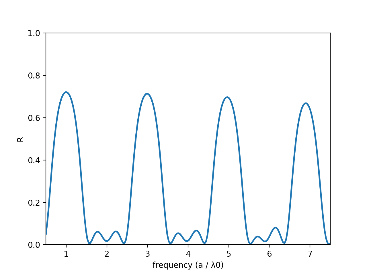
We can keep adding layers and adding layers to our heart's content. If we add another 6 layers, the plot will look something like this:
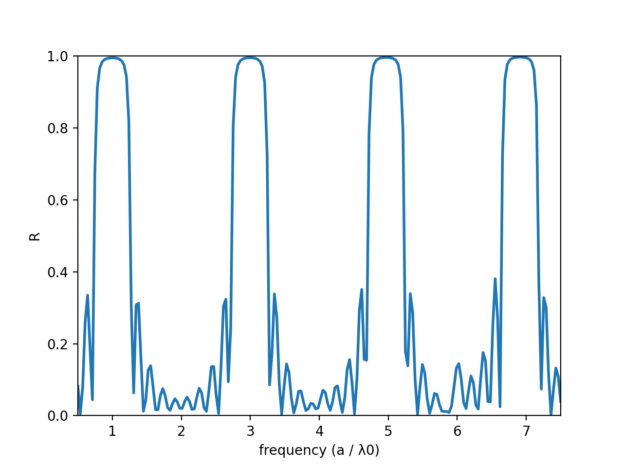
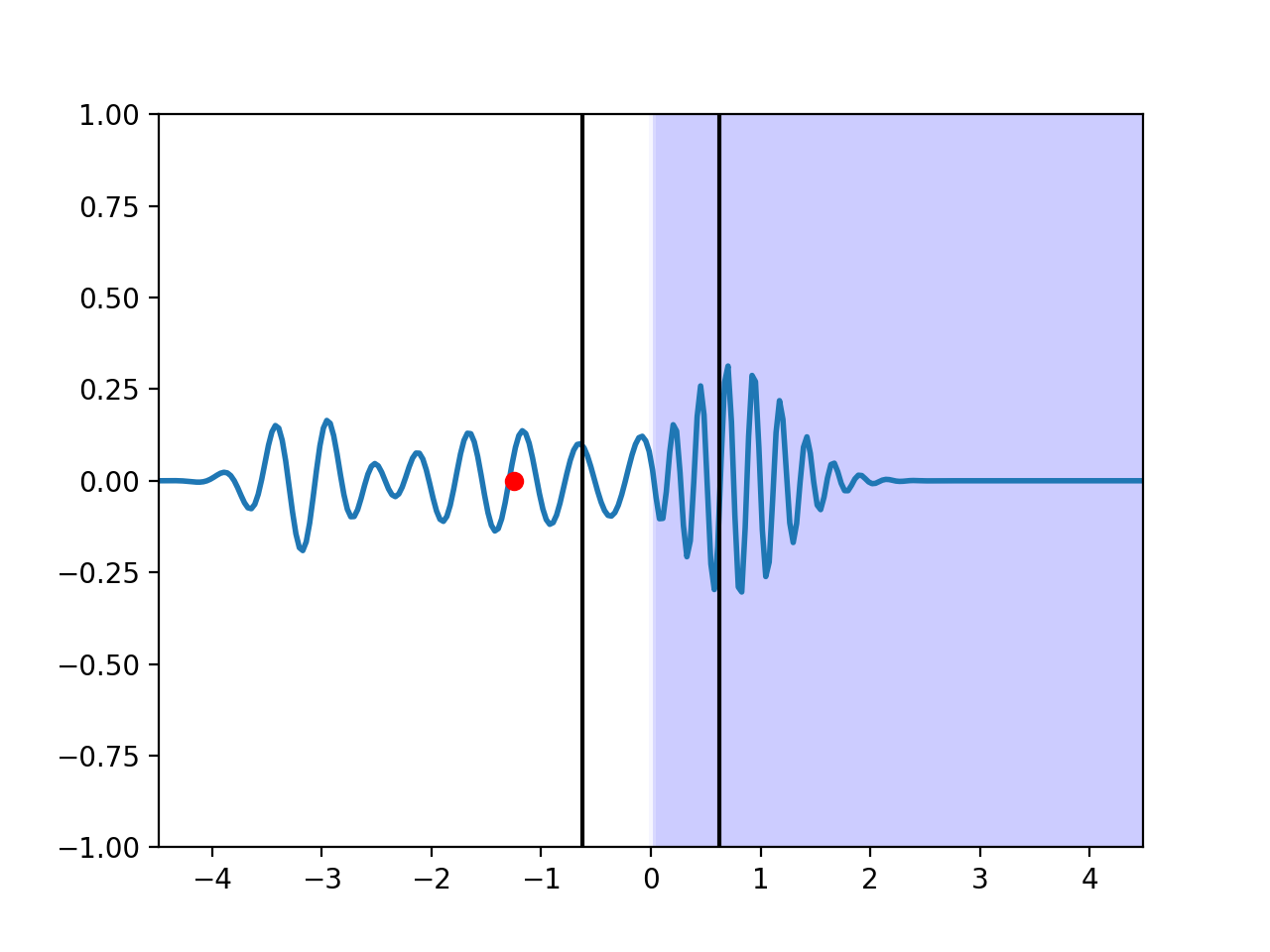
As you can see the reflection spectra is getting closer and closer to 1 at the maxima (and if we added an infinite number of layers it would be exactly 1). This is neat. To get a better feel for what's happening, let's run a narrower-bandwidth simulation near one of the maxima (so say at f = 3), and see what a plane wave getting reflected by this mirror actually looks like (I've moved the source a little to the left and greatly increased the propagation distance so we can better see what's going on):
It looks like some of the pulse is penetrating into the first layer, but the amplitude of the pulse is decaying more and more as we go further into each layer, with a very small amount leaking all the way through. We also see that as the wave reflects, it forms a standing wave, and eventually most of the pulse leaves the mirror from the direction it came.
Now that we know how to create mirrors, we can use them to create devices - probably the most important devices in all of electromagnetics (other than waveguides) - resonators. This will be the subject of the next lesson.
Full Code
You can also download the code here.
import meep as mp
import numpy as np
import matplotlib.pyplot as plt
from matplotlib import animation

resolution = 120
frequency = 4.0
frequencyWidth = 7.0
numberFrequencies = 200
pmlThickness = 2.0
animationTimestepDuration = 0.05
powerDecayTarget = 1e-9
t1 = 0.125
t2 = 0.25
n1 = 2.0
n2 = 1.0
ns = 1.3
ts = 0.25

layerIndexes = np.array([1.0, n1, n2, n1, n2, n1, n2, n1, n2, n1, ns])
layerThicknesses = np.array([50, t1, t2, t1, t2, t1, t2, t1, t2, t1, ts])
layerThicknesses[0] += pmlThickness
layerThicknesses[-1] += pmlThickness
length = np.sum(layerThicknesses)
layerCenters = np.cumsum(layerThicknesses) - layerThicknesses/2
layerCenters = layerCenters - length/2

sourceLocation = mp.Vector3(0, 0, layerCenters[0] - layerThicknesses[0]/4)
transmissionMonitorLocation = mp.Vector3(0, 0, layerCenters[-1]-pmlThickness/2)
reflectionMonitorLocation = mp.Vector3(0, 0, layerCenters[0] + layerThicknesses[0]/4)

cellSize = mp.Vector3(0, 0, length)

sources = [mp.Source(
    mp.GaussianSource(frequency=frequency,fwidth=frequencyWidth),
    component=mp.Ex,
    center=sourceLocation)
    ]

geometry = [mp.Block(mp.Vector3(mp.inf, mp.inf, layerThicknesses[i]),
    center=mp.Vector3(0, 0, layerCenters[i]), material=mp.Medium(index=layerIndexes[i]))
    for i in range(layerThicknesses.size)]

pmlLayers = [mp.PML(thickness=pmlThickness)]

simulation = mp.Simulation(
    cell_size=cellSize,
    sources=sources,
    resolution=resolution,
    dimensions=1,
    boundary_layers=pmlLayers)

incidentRegion = mp.FluxRegion(center=reflectionMonitorLocation)
incidentFluxMonitor = simulation.add_flux(frequency, frequencyWidth, numberFrequencies, incidentRegion)

simulation.run(until_after_sources=mp.stop_when_fields_decayed(20, mp.Ex,
    transmissionMonitorLocation, powerDecayTarget))
fieldEx = np.real(simulation.get_array(center=mp.Vector3(0, 0, 0), size=cellSize, component=mp.Ex))
fieldData = np.zeros(len(fieldEx))

incidentFluxToSubtract = simulation.get_flux_data(incidentFluxMonitor)

simulation = mp.Simulation(
    cell_size=cellSize,
    sources=sources,
    resolution=resolution,
    boundary_layers=pmlLayers,
    dimensions=1,
    geometry=geometry)

transmissionRegion = mp.FluxRegion(center=transmissionMonitorLocation)
transmissionFluxMonitor = simulation.add_flux(frequency, frequencyWidth, numberFrequencies, transmissionRegion)
reflectionRegion = incidentRegion
reflectionFluxMonitor = simulation.add_flux(frequency, frequencyWidth, numberFrequencies, reflectionRegion)
simulation.load_minus_flux_data(reflectionFluxMonitor, incidentFluxToSubtract)

def updateField(sim):
    global fieldData
    fieldEx = np.real(sim.get_array(center=mp.Vector3(0, 0, 0), size=cellSize, component=mp.Ex))
    fieldData = np.vstack((fieldData, fieldEx))

simulation.run(mp.at_every(animationTimestepDuration, updateField),
        until_after_sources=mp.stop_when_fields_decayed(20, mp.Ex,
            transmissionMonitorLocation, powerDecayTarget))

incidentFlux = np.array(mp.get_fluxes(incidentFluxMonitor))
transmittedFlux = np.array(mp.get_fluxes(transmissionFluxMonitor))
reflectedFlux = np.array(mp.get_fluxes(reflectionFluxMonitor))
R = -reflectedFlux / incidentFlux
T = transmittedFlux / incidentFlux
#print(T)
#print(R)
print(R + T)

frequencies = np.array(mp.get_flux_freqs(reflectionFluxMonitor))
reflectionSpectraFigure = plt.figure()
reflectionSpectraAxes = plt.axes(xlim=(frequency-frequencyWidth/2, frequency+frequencyWidth/2),ylim=(0, 1))
reflectionLine, = reflectionSpectraAxes.plot(frequencies, R, lw=2)
reflectionSpectraAxes.set_xlabel('frequency (a / \u03BB0)')
reflectionSpectraAxes.set_ylabel('R')
plt.show()

(x, y, z, w) = simulation.get_array_metadata()
indexArray = np.sqrt(simulation.get_epsilon())

fig = plt.figure()
ax = plt.axes(xlim=(min(z),max(z)),ylim=(-1,1))
line, = ax.plot([], [], lw=2)

colorArray = indexArray - 1 # make sure free space shows up as white
if(colorArray.max() > 0):
    colorArray = colorArray / colorArray.max() # normalize the color array so that the max index shows up dark blue
for i in range(len(indexArray) - 1):
    ax.fill_between([z[i], z[i+1]], [-1, -1], [1, 1],
            color=(1-colorArray[i],1-colorArray[i],1), linewidth=0.0, alpha=0.2)
ax.plot(sourceLocation.z, 0, 'ro')
ax.axvline(transmissionMonitorLocation.z, ymin=-1, color='black')
ax.axvline(reflectionMonitorLocation.z, ymin=-1, color='black')

def init():
    line.set_data([],[])
    return line,

def animate(i):
    line.set_data(z, fieldData[i])
    return line,

numberAnimationTimesteps = fieldData.shape[0]
fieldAnimation = animation.FuncAnimation(fig, animate, init_func=init,
        frames=numberAnimationTimesteps, interval=20, blit=True)

#fieldAnimation.save('basic_animation.mp4', fps=30, extra_args=['-vcodec', 'libx264'])
plt.show()
A quiz question
If you found this content helpful, it would mean a lot to me if you would support me on Patreon. Help keep this content ad-free, get access to my Discord server, exclusive content, and receive my personal thanks for as little as $2. :)
Become a Patron!