
Computational Electromagnetics with MEEP Part 2: 1D MEEP

Lesson 10: Thin-Film Interference
Now on to the fun stuff!
Not that reflection off an interface isn't fun, but now we get to actually use what we've learned in the previous lessons to see cool effects, like thin-film interference, the subject of this lesson. This also is an excellent starting point for the study of mirrors, anti-reflection coatings, and resonant devices, which are the subject of the next several lessons, and will wrap up our one-dimensional adventures in MEEP (then onto 2 dimensions!). The basic idea we want to simulate in this lesson is a thin film on a surface - I'm going to choose oil on water, because it's as good a starting point as any. Let's take a look at what we want our simulation to look like:

Let's do this at normal incidence to simplify things - if you wanted to perform the simulation over multiple angles and frequencies you now know how to do that :). Oil also doesn't really have a refractive index of 2, it's closer to 1.5, but it makes the math easier. For now, let's pretend that these materials index of refraction doesn't depend on wavelength (a bad assumption, but a good starting point). The setup of the simulation is pretty much identical to all our previous simulations, but now we have an extra Block() object in our geometry variable, and the position/index of our second material are different, because we need to accomodate the film.
geometry = [mp.Block(
    mp.Vector3(mp.inf, mp.inf, filmThickness),
    center=mp.Vector3(0, 0, filmThickness/2),
    material=mp.Medium(index=2)),
    mp.Block(
    mp.Vector3(mp.inf, mp.inf, materialThickness + pmlThickness),
    center=mp.Vector3(0, 0, filmThickness + materialThickness/2 + pmlThickness/2),
    material=mp.Medium(index=1.3))]
The only thing we need is the thickness of the film. What should we make it? Ideally we would like to see some easily-recognizable feature of the spectrum, like a maxima or a minima, somewhere in our tested frequency range (which I will keep at 1.5 to 2.5 for now). Constructive interference, or when we have a maxima in our reflectance spectrum, occurs when the thickness is equal to \(\left(m - \frac{1}{2}\right)\frac{\lambda_0}{2 n}\), where \(m\) is an integer (at least one) and \(n\) is the refractive index of the film (in our case, 2). Destructive interference on the other hand, when the reflectance is at a minimum, occurs when the thickness is equal to \(m*\frac{\lambda_0}{2 n}\). If we put everything in MEEP coordinates, we get that:
\(t_{MEEP} = \left(m-\frac{1}{2}\right)*\frac{1}{2 n f_{MEEP}}\) (constructive)
\(t_{MEEP} = m*\frac{1}{2 n f_{MEEP}}\) (destructive)
Since \(n=2\), and our center frequency is also 2, if we make our thickness 0.125, we should see destructive interference right at our center frequency. Is that what we see? Let's plot the reflection spectra of this oil-water system when we send a plane wave in from the air region. If you don't remember how to do that, don't worry, it's in a previous lesson :). Since our maximum frequency is 2.5 and our maximum index is 2, let's use a resolution of 40 to get at least 8 points per wavelength at all frequencies. If you don't remember how to choose the resolution, you can find that in this lesson.
Plotting the reflection spectra, it looks like this:
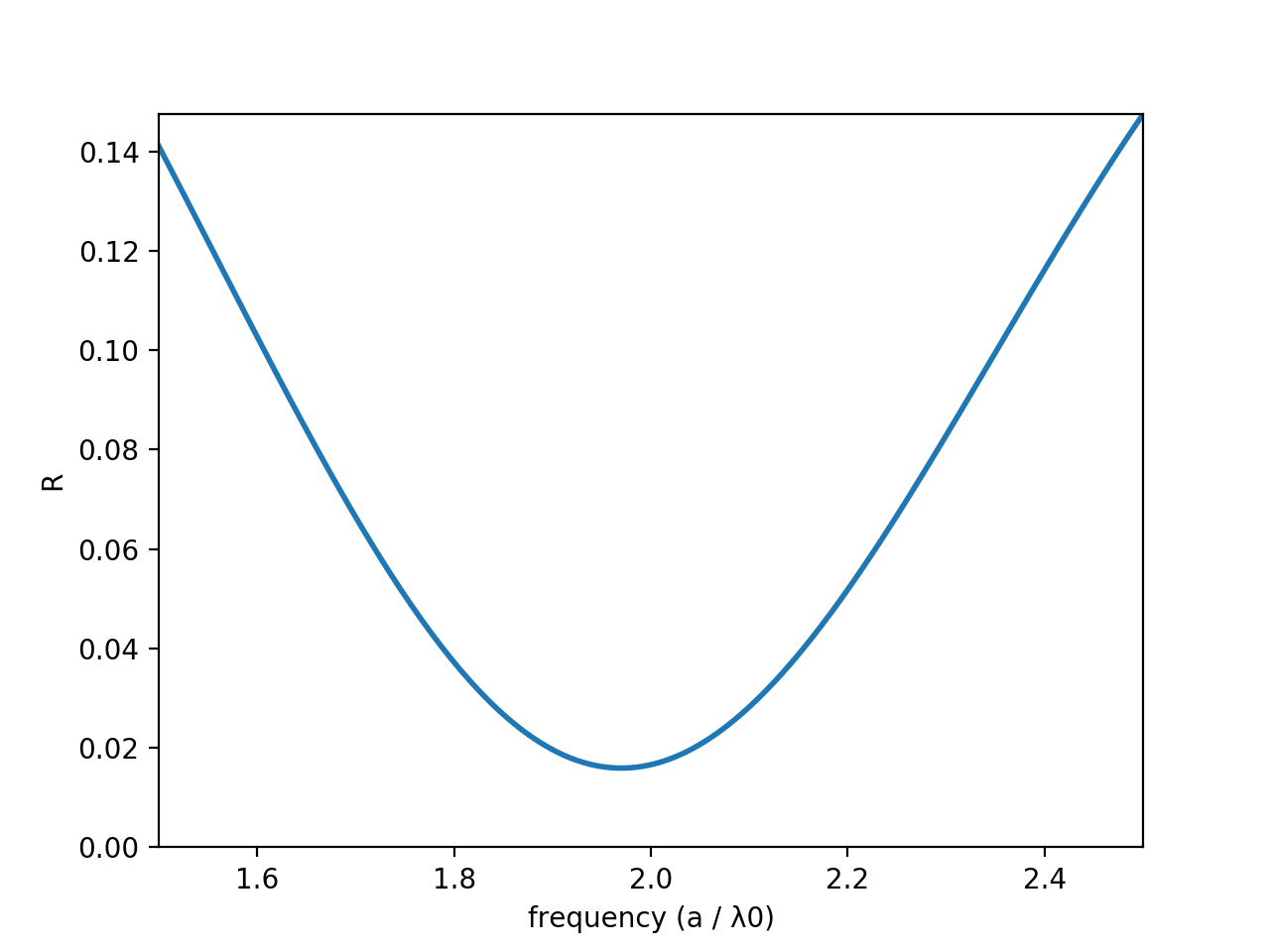
Does this make sense? Almost. It looks like the minimum is slightly shifted compared to what it should be (1.96 instead of 2). Let's see if doubling the resolution makes this better. If you double the resolution, you will find that, indeed, the new center frequency is about 1.98. Doubling it again will get it even closer, to ~1.995. Great! Our simulation is converging. Let's drop our resolution back down to 40. Now, what about other values of m? We should get destructive interference not just at \(m = 1\), but also \(m = 2, 3\), and so on. Let's increase our frequency to encompass frequencies from 1.5 to 7.5 so that we can see the first three minima.
What should the center frequency and the width be changed to so that we span frequencies from 1.5 to 7.5?
Ok, what happens when we plot this? Let's take a look:
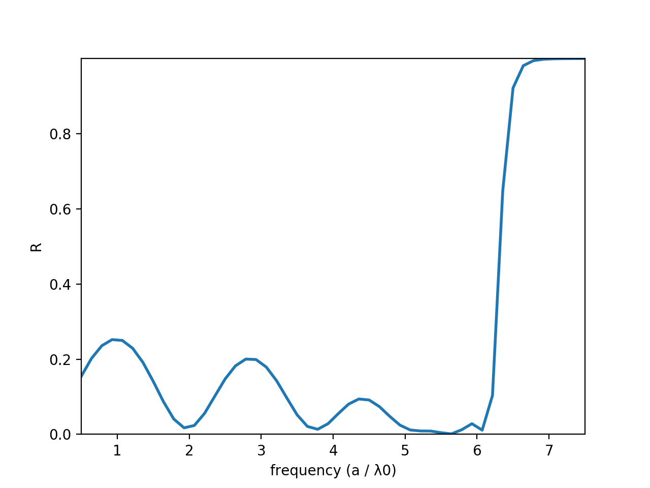
What on earth is this monstrosity? It's all kinds of ugly - it has the minima around 2, and one that kinda looks like it's near 4, along with the maxima at 1, 3, and 5 (ish?). What is going on...?
What is going on with the simulation?
Ah! We are working with higher frequencies now, we need to adjust the resolution. Let's also increase the number of frequencies to 200 so the plot doesn't look so choppy.
What is the minimum resolution we should choose if our frequencies span the range of 1.5 to 7.5?
Now, let's plot what this looks like:
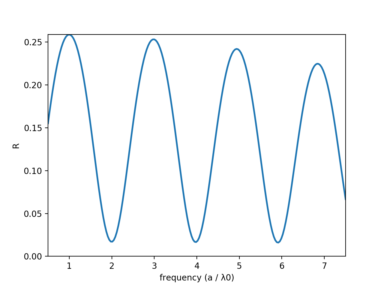
Ah, that's better. The minima are right where we expect them, as are the maxima. But the plot is still sloping downward... do we expect that? In this simple case, no, but often we won't know the answer to that question. How can we figure out whether this is an artifact of our simulation or not?
How can we figure out whether this sloping graph is an artifact of our simulation?
Brilliant idea! Let's give it a try, doubling the resolution:
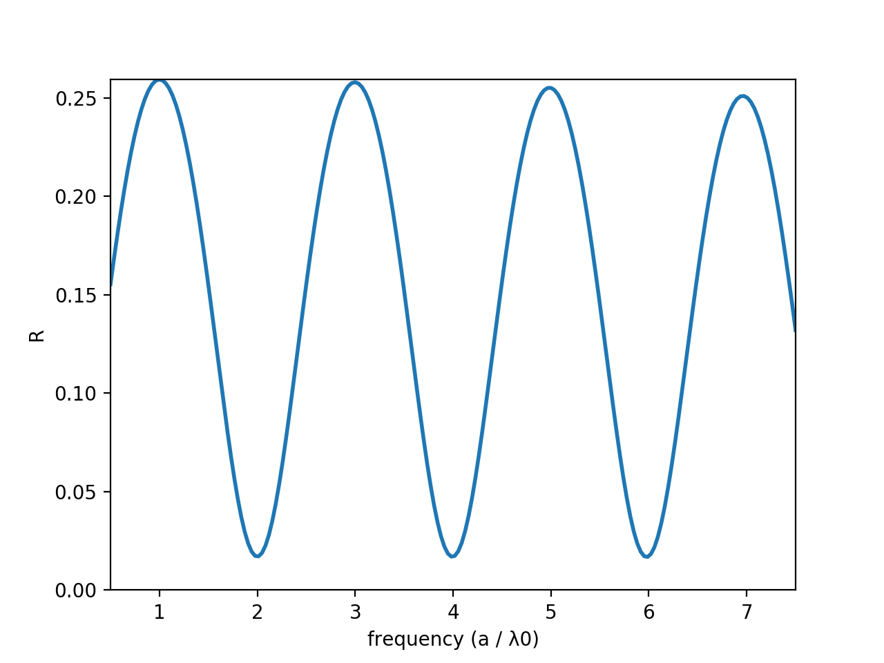
As you can see above, the downward sloping has been greatly reduced. If we were to increase our resolution further, we could eliminate it almost entirely.
In this practical example, we saw with our own eyes how critically important convergence testing was. If we hadn't done any convergence testing, and taken the first reflectance spectra at face value, we would have an answer that is qualitatively and quantitatively completely different from the correct answer. It is always critical, for this reason, to do convergence testing. In the next lesson, we will take thin-film interference to an extreme - with the dielectric mirror.
Full Code
As usual, you can download the code here, or find it below:
import meep as mp
import numpy as np
import matplotlib.pyplot as plt

resolution = 120
frequency = 4.0
frequencyWidth = 7
numberFrequencies = 200
pmlThickness = 2.0
animationTimestepDuration = 0.05
filmThickness = 0.125
materialThickness = 2.5
length = 2 * materialThickness + filmThickness +  2 * pmlThickness
powerDecayTarget = 1e-9
transmissionMonitorLocation = mp.Vector3(0, 0, materialThickness/4)
theta = np.radians(0)
kVector = mp.Vector3(np.sin(theta), 0, np.cos(theta)).scale(frequency - frequencyWidth/2)

cellSize = mp.Vector3(0, 0, length)

sources = [mp.Source(
    mp.GaussianSource(frequency=frequency,fwidth=frequencyWidth),
    component=mp.Ex,
    center=mp.Vector3(0, 0, -materialThickness/2)),
    ]

geometry = [mp.Block(
    mp.Vector3(mp.inf, mp.inf, filmThickness),
    center=mp.Vector3(0, 0, filmThickness/2),
    material=mp.Medium(index=2)),
    mp.Block(
    mp.Vector3(mp.inf, mp.inf, materialThickness + pmlThickness),
    center=mp.Vector3(0, 0, filmThickness + materialThickness/2 + pmlThickness/2),
    material=mp.Medium(index=1.3))]

pmlLayers = [mp.PML(thickness=pmlThickness, R_asymptotic=1e-35)]

simulation = mp.Simulation(
    cell_size=cellSize,
    sources=sources,
    resolution=resolution,
    boundary_layers=pmlLayers,
    k_point=kVector)

incidentRegion = mp.FluxRegion(center=mp.Vector3(0, 0, -materialThickness/4))
incidentFluxMonitor = simulation.add_flux(frequency, frequencyWidth, numberFrequencies, incidentRegion)

simulation.run(
    until_after_sources=mp.stop_when_fields_decayed(20, mp.Ex,
    transmissionMonitorLocation, powerDecayTarget))

incidentFluxToSubtract = simulation.get_flux_data(incidentFluxMonitor)

simulation = mp.Simulation(
    cell_size=cellSize,
    sources=sources,
    resolution=resolution,
    boundary_layers=pmlLayers,
    geometry=geometry,
    k_point=kVector)

transmissionRegion = mp.FluxRegion(center=transmissionMonitorLocation)
transmissionFluxMonitor = simulation.add_flux(frequency, frequencyWidth, numberFrequencies, transmissionRegion)
reflectionRegion = incidentRegion
reflectionFluxMonitor = simulation.add_flux(frequency, frequencyWidth, numberFrequencies, reflectionRegion)
simulation.load_minus_flux_data(reflectionFluxMonitor, incidentFluxToSubtract)

simulation.run(mp.at_every(animationTimestepDuration, updateField),
        #until=endTime)
        until_after_sources=mp.stop_when_fields_decayed(20, mp.Ex,
            transmissionMonitorLocation, powerDecayTarget))

incidentFlux = np.array(mp.get_fluxes(incidentFluxMonitor))
transmittedFlux = np.array(mp.get_fluxes(transmissionFluxMonitor))
reflectedFlux = np.array(mp.get_fluxes(reflectionFluxMonitor))
R = -reflectedFlux / incidentFlux
T = transmittedFlux / incidentFlux
print(T)
print(R)
print(R + T)

frequencies = np.array(mp.get_flux_freqs(reflectionFluxMonitor))
reflectionSpectraFigure = plt.figure()
reflectionSpectraAxes = plt.axes(xlim=(frequency-frequencyWidth/2, frequency+frequencyWidth/2),ylim=(0, R.max()))
reflectionLine, = reflectionSpectraAxes.plot(frequencies, R, lw=2)
reflectionSpectraAxes.set_xlabel('frequency (a / \u03BB0)')
reflectionSpectraAxes.set_ylabel('R')
plt.show()
If you found this content helpful, it would mean a lot to me if you would support me on Patreon. Help keep this content ad-free, get access to my Discord server, exclusive content, and receive my personal thanks for as little as $2. :)
Become a Patron!