Computational Electromagnetics with MEEP Part 2: 1D MEEP

Lesson 9: Multi-Frequency, Multi-Angle Simulations
All the simulations!
In the previous lesson, we saw that if we want several frequencies at a single angle of incidence, we must do a bunch of simulations at different angles of incidence, because of we have several frequencies in one simulation we necessarily have different corresponding angles.
So how do we do that? Let's start with the code from two lessons ago, and modify it to suit our needs. First, we'll want to make sure to scale the k-vector to the minimum frequency instead of the center frequency, as we discussed in the last lesson. First, I'm going to delete all the code that has to do with recording the field data (comment it out instead or create a new file if this makes you queasy). This is just because since we want to run a bunch of simulations, recording the field each time and plotting it is going to slow us down quite a bit. And we all have better things to do with our lives than sit around and wait for our simulators to do our bidding.
We're also going to put everything to do with actually running our simulations inside a single function, so that we can run it a bunch of times. This function should take as an argument the angle, in degrees, that we want to run the simulation at, and then run the necessary simulation(s) and give us back the values of \(R\) and \(T\) at each frequency, along with the angles those correspond to. We could compute those latter ones separately, but I think this is simpler. I've called the function runSimulation() (because I'm creative like that):
def runSimulation(thetaDegrees):
    thetaRadians = np.radians(thetaDegrees)
    kVector = mp.Vector3(np.sin(thetaRadians), 0, np.cos(thetaRadians)).scale(minimumFrequency)
    simulation = mp.Simulation(
        cell_size=cellSize,
        sources=sources,
        resolution=resolution,
        boundary_layers=pmlLayers,
        k_point=kVector)

    incidentFluxMonitor = simulation.add_flux(frequency, frequencyWidth, numberFrequencies, incidentRegion)

    simulation.run(until_after_sources=mp.stop_when_fields_decayed(20, mp.Ex,
        transmissionMonitorLocation, powerDecayTarget))

    incidentFluxToSubtract = simulation.get_flux_data(incidentFluxMonitor)

    simulation = mp.Simulation(
        cell_size=cellSize,
        sources=sources,
        resolution=resolution,
        boundary_layers=pmlLayers,
        geometry=geometry,
    k_point=kVector)

    transmissionRegion = mp.FluxRegion(center=transmissionMonitorLocation)
    transmissionFluxMonitor = simulation.add_flux(frequency, frequencyWidth, numberFrequencies, transmissionRegion)
    reflectionRegion = incidentRegion
    reflectionFluxMonitor = simulation.add_flux(frequency, frequencyWidth, numberFrequencies, reflectionRegion)
    simulation.load_minus_flux_data(reflectionFluxMonitor, incidentFluxToSubtract)

    simulation.run(until_after_sources=mp.stop_when_fields_decayed(20, mp.Ex,
                transmissionMonitorLocation, powerDecayTarget))

    incidentFlux = np.array(mp.get_fluxes(incidentFluxMonitor))
    transmittedFlux = np.array(mp.get_fluxes(transmissionFluxMonitor))
    reflectedFlux = np.array(mp.get_fluxes(reflectionFluxMonitor))
    R = np.array(-reflectedFlux / incidentFlux)
    T = np.array(transmittedFlux / incidentFlux)

    frequencies = np.array(mp.get_flux_freqs(reflectionFluxMonitor))
    kx = kVector.x
    angles = np.arcsin(kx/frequencies)

    return angles, frequencies, R, T
First, we ened to choose the different angles we will be running this function at. Let's set our maximum angle to 85, with a minimum angle of 0, and increment the angle in units of 5 degrees. You can choose whatever you want, but I think this is a good starting point:
angleIncrement = 5
angleMin = 0
angleMax = 10
anglesToTest = np.arange(angleMin, angleMax + angleIncrement, angleIncrement)
Now comes a bit of a tricky part. Since we have a several different angles and many different frequencies, our data is two-dimensional. But while the frequency data is evenly spaced, the angular data is some awkward contortion of arcsin of stuff multiplied by sin. So we can't just record the data \(R\) and \(T\) by itself in a 2D array, we have to also record the value of \(f\) and \(\theta\) that each of those \(R\) and \(T\) came from. So we actually want four 2D arrays. One for \(R\), one for \(T\), one for the value of \(\theta\) for each of those, and one for the value of \(f\). Fortunately, we already know the size of these 2D arrays - just the number of angles by the number of frequencies.
angleGrid = np.zeros((len(anglesToTest), numberFrequencies))
frequencyGrid = np.zeros((len(anglesToTest), numberFrequencies))
RGrid = np.zeros((len(anglesToTest), numberFrequencies))
TGrid = np.zeros((len(anglesToTest), numberFrequencies))
Now that all our variables are set up, we can just run the simulation with a bunch of different angles, and plop the data in the appropriate variables:
i = 0;
for theta in anglesToTest:
    angles, frequencies, R, T = runSimulation(theta)
    angleGrid[i] = np.degrees(angles)
    frequencyGrid[i] = frequencies
    RGrid[i] = R
    TGrid[i] = T
    i = i + 1
To make sure everything makes sense, let's print \(R+T\) to the screen (as long as all the values are close to 1, energy conservation holds and nothing went horribly wrong).
CGrid = RGrid + TGrid
print(CGrid) # make sure that conservation of energy holds for all frequencies tested.
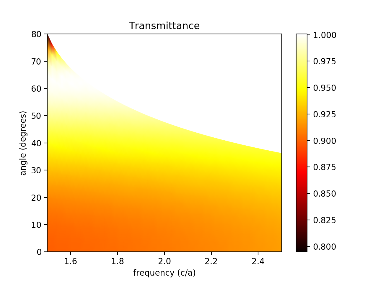
And that's it! We've got all our data. All that's left is to visualize it and make sure it's not hopelessly wrong. To do this we're going to use matplotlib's "pcolormesh", which takes the angle and frequency grids we generated before and plots the value of \(R\) or \(T\) using a heatmap:
plt.figure()
plt.pcolormesh(frequencyGrid, angleGrid, TGrid, cmap='hot', shading='gouraud', vmin=TGrid.min(), vmax=TGrid.max())
plt.xlabel("frequency (c/a)")
plt.ylabel("angle (degrees)")
plt.title("Transmittance")
cbar = plt.colorbar()
plt.show()
Do our results make sense? Let's check a couple things. First, does conservation of energy hold? It looks like for the most part, yes, although there are some data points in the 80-degree simulation (the first couple) that have \(R+T\) of ~0.95, so I wouldn't trust that data. That corresponds to the awkward-looking smear in the upper left. How else can we check if this data makes sense? Well, one distinguishing feature we can look for, since this is a p-polarized EM wave, is Brewster's Angle, at which the transmittance should become 1. We we expect to find it at \(tan^{-1}\left(n_2/n_1\right)\), or about 63 degrees. We do indeed see the transmittance go to 1 at what looks like an angle of 63 degrees. What about the rest of the plot? Do we expect the transmittance to depend on frequency? As in a previou lesson, no, we don't, because our refractive index is not a function of wavelength. It looks like this graph isn't perfectly constant over frequency at a given angle. For this and the smudge in the upper-left, I don't really love this plot. Let's try with higher resolutions.
After trying resolutions of 64 and 128, the smudge doesn't look a whole lot better, but the graph looks more frequency-independent. We could try increasing the size of the PML or increasing the distance from the source to the PML, but that corner corresponds to frequencies on the edge of our distribution, which have very low amplitudes and high error in the first place. If we want data from that corner, we should run a simulation at a different (lower) center frequency.
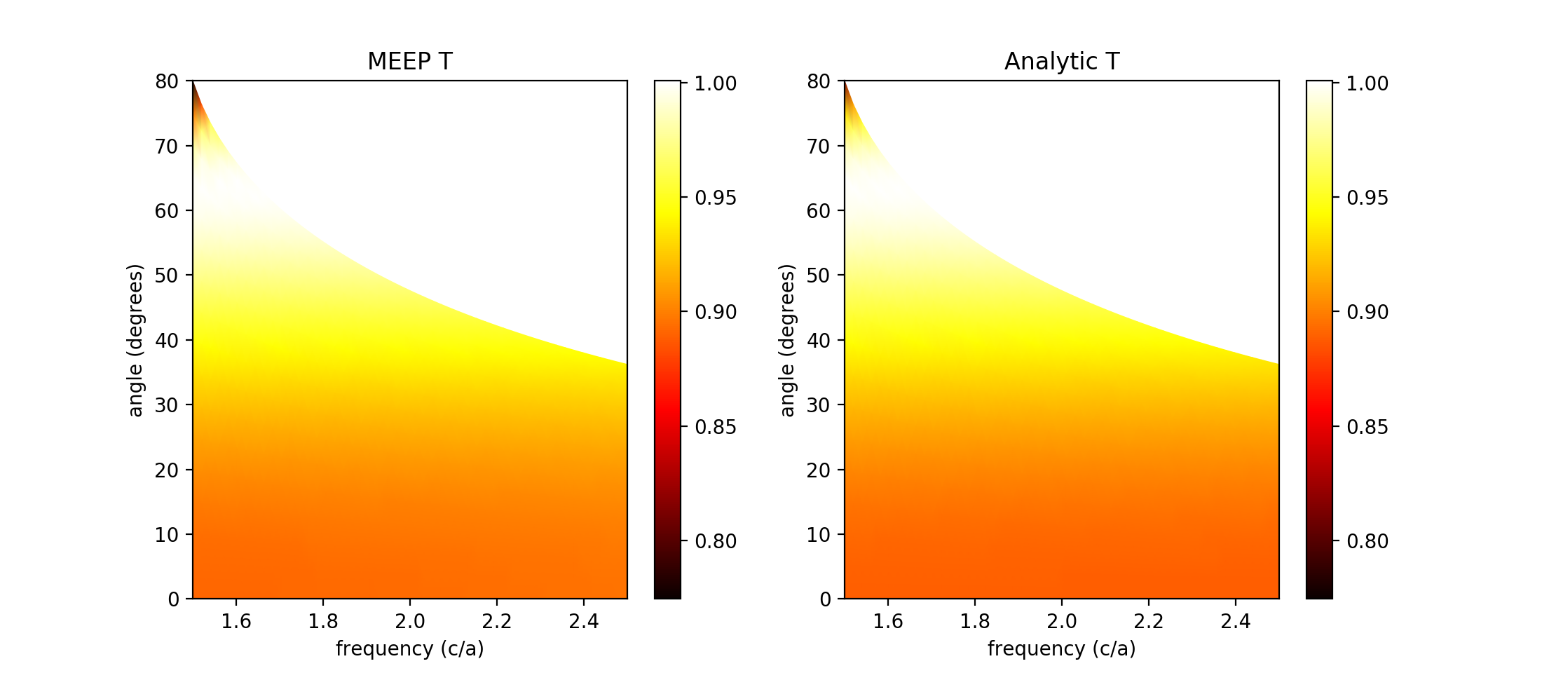
There's one more thing we could do to check if our data makes sense - we could actually plot the known values of the transmission coefficient using Fresnel's equations, using the angles we already generated.
\(T_p = 1 - |\frac{n_1 cos\theta_2 - n_2 cos\theta_1}{n_1 cos\theta_2 + n_2 cos\theta_1}|^2\)
We can write a function that does this, and then create a new variable that calculates the value of \(T\) everywhere we have a value from MEEP:
def Tp(theta1Degrees):
    theta1 = np.radians(theta1Degrees)
    theta2 = np.arcsin(n1/n2 *np.sin(theta1))
    return 1 - np.square(np.abs( (n1*np.cos(theta2) - n2*np.cos(theta1)) / (n1*np.cos(theta2) + n2*np.cos(theta1))))
TAnalyticGrid = Tp(angleGrid)
Now, to change the code to plot both figures side by side, you will have to tweak the plotting function a bit (I've posted it below and took it from matplotlib's documentation).
fig, (simulationAxes, analyticAxes) = plt.subplots(ncols=2)

analyticPlot = analyticAxes.pcolormesh(frequencyGrid, angleGrid, TAnalyticGrid,
        cmap='hot', shading='gouraud', vmin=TGrid.min(), vmax=TGrid.max())
analyticAxes.set_title('Analytic T')
fig.colorbar(analyticPlot,  ax=analyticAxes)
analyticAxes.set_xlabel("frequency (c/a)")
analyticAxes.set_ylabel("angle (degrees)")


simulationPlot = simulationAxes.pcolormesh(frequencyGrid, angleGrid, TGrid,
        cmap='hot', shading='gouraud', vmin=TGrid.min(), vmax=TGrid.max())
simulationAxes.set_title('MEEP T')
fig.colorbar(simulationPlot, ax=simulationAxes)
simulationAxes.set_xlabel("frequency (c/a)")
simulationAxes.set_ylabel("angle (degrees)")

plt.show()
Now, if you run the code in ets entirety, you will get two plots, side-by-side:
Those plots look pretty darn similar to me. Except for the smudge in the upper-left I can't tell them apart.
Awesome. We now know how to simulate and plot reflection and transmission spectra as a function of frequency and angle for an interface. In the next lesson, we will build on what we learned here and investigate a case where we do have wavelength dependence of our reflection and transmission spectra - thin-film interference.
Full Code
Download the full code for this lesson here, or see it below:
import meep as mp
import numpy as np
import matplotlib.pyplot as plt
from matplotlib import animation

resolution = 64
frequency = 2.0
frequencyWidth = 1
minimumFrequency = frequency - frequencyWidth/2
numberFrequencies = 50
pmlThickness = 4.0
animationTimestepDuration = 0.05
materialThickness = 2.5
length = 2 * materialThickness + 2 * pmlThickness
powerDecayTarget = 1e-9
transmissionMonitorLocation = mp.Vector3(0, 0, materialThickness/4)

cellSize = mp.Vector3(0, 0, length)

sources = [mp.Source(
    mp.GaussianSource(frequency=frequency,fwidth=frequencyWidth),
    component=mp.Ex,
    center=mp.Vector3(0, 0, -materialThickness/2)),
    ]

geometry = [mp.Block(
    mp.Vector3(mp.inf, mp.inf, materialThickness + pmlThickness),
    center=mp.Vector3(0, 0, materialThickness/2 + pmlThickness/2),
    material=mp.Medium(index=2))]

pmlLayers = [mp.PML(thickness=pmlThickness)]

incidentRegion = mp.FluxRegion(center=mp.Vector3(0, 0, -materialThickness/4))

def runSimulation(thetaDegrees):
    thetaRadians = np.radians(thetaDegrees)
    kVector = mp.Vector3(np.sin(thetaRadians), 0, np.cos(thetaRadians)).scale(minimumFrequency)
    simulation = mp.Simulation(
        cell_size=cellSize,
        sources=sources,
        resolution=resolution,
        boundary_layers=pmlLayers,
        k_point=kVector)

    incidentFluxMonitor = simulation.add_flux(frequency, frequencyWidth, numberFrequencies, incidentRegion)

    simulation.run(until_after_sources=mp.stop_when_fields_decayed(20, mp.Ex,
        transmissionMonitorLocation, powerDecayTarget))

    incidentFluxToSubtract = simulation.get_flux_data(incidentFluxMonitor)

    simulation = mp.Simulation(
        cell_size=cellSize,
        sources=sources,
        resolution=resolution,
        boundary_layers=pmlLayers,
        geometry=geometry,
    k_point=kVector)

    transmissionRegion = mp.FluxRegion(center=transmissionMonitorLocation)
    transmissionFluxMonitor = simulation.add_flux(frequency, frequencyWidth, numberFrequencies, transmissionRegion)
    reflectionRegion = incidentRegion
    reflectionFluxMonitor = simulation.add_flux(frequency, frequencyWidth, numberFrequencies, reflectionRegion)
    simulation.load_minus_flux_data(reflectionFluxMonitor, incidentFluxToSubtract)

    simulation.run(until_after_sources=mp.stop_when_fields_decayed(20, mp.Ex,
                transmissionMonitorLocation, powerDecayTarget))

    incidentFlux = np.array(mp.get_fluxes(incidentFluxMonitor))
    transmittedFlux = np.array(mp.get_fluxes(transmissionFluxMonitor))
    reflectedFlux = np.array(mp.get_fluxes(reflectionFluxMonitor))
    R = np.array(-reflectedFlux / incidentFlux)
    T = np.array(transmittedFlux / incidentFlux)

    frequencies = np.array(mp.get_flux_freqs(reflectionFluxMonitor))
    kx = kVector.x
    angles = np.arcsin(kx/frequencies)

    return angles, frequencies, R, T

angleIncrement = 5
angleMin = 0
angleMax = 80
anglesToTest = np.arange(angleMin, angleMax + angleIncrement, angleIncrement)

angleGrid = np.zeros((len(anglesToTest), numberFrequencies))
frequencyGrid = np.zeros((len(anglesToTest), numberFrequencies))
RGrid = np.zeros((len(anglesToTest), numberFrequencies))
TGrid = np.zeros((len(anglesToTest), numberFrequencies))

i = 0;
for theta in anglesToTest:
    angles, frequencies, R, T = runSimulation(theta)
    angleGrid[i] = np.degrees(angles)
    frequencyGrid[i] = frequencies
    RGrid[i] = R
    TGrid[i] = T
    i = i + 1

CGrid = RGrid + TGrid
print(CGrid) # make sure that conservation of energy holds for all frequencies tested.

fig, (simulationAxes, analyticAxes) = plt.subplots(ncols=2)

analyticPlot = analyticAxes.pcolormesh(frequencyGrid, angleGrid, TAnalyticGrid,
        cmap='hot', shading='gouraud', vmin=TGrid.min(), vmax=TGrid.max())
analyticAxes.set_title('Analytic T')
fig.colorbar(analyticPlot,  ax=analyticAxes)
analyticAxes.set_xlabel("frequency (c/a)")
analyticAxes.set_ylabel("angle (degrees)")


simulationPlot = simulationAxes.pcolormesh(frequencyGrid, angleGrid, TGrid,
        cmap='hot', shading='gouraud', vmin=TGrid.min(), vmax=TGrid.max())
simulationAxes.set_title('MEEP T')
fig.colorbar(simulationPlot, ax=simulationAxes)
simulationAxes.set_xlabel("frequency (c/a)")
simulationAxes.set_ylabel("angle (degrees)")

plt.show()
If you found this content helpful, it would mean a lot to me if you would support me on Patreon. Help keep this content ad-free, get access to my Discord server, exclusive content, and receive my personal thanks for as little as $2. :)
Become a Patron!

